Region Topic Analysis

This tutorial covers topic modeling analysis with TF-MInDi:

• Running topic modeling on regions using run_topic_modeling()

• Evaluating different topic numbers with evaluate_topic_models()

• Analyzing topic-cluster and topic-DBD relationships

• Visualizing topics in t-SNE space and heatmaps

import tfmindi as tm

DATA_DIR = "../../../../data/tfmindi/"

# Load clustered data from previous tutorial
adata = tm.load_h5ad(DATA_DIR + "seqlets_clustered.h5ad")

Running Topic Modeling

Topic modeling helps discover co-occurring TF binding patterns across genomic regions. We use run_topic_modeling() which applies Latent Dirichlet Allocation (LDA) to find topics based on seqlet cluster compositions.

Each region gets a topic probability distribution, and each topic represents a pattern of co-occurring TF binding clusters.

The results of the topic modeling will be stored in our anndata.uns["topic_modeling"].

# Run topic modeling with 15 topics
tm.tl.run_topic_modeling(adata, n_topics=15, random_state=42)

Filtered 0 seqlets with unknown DBD annotations
Using 679653 deduplicated seqlets across 37265 regions
Count matrix shape: (37265, 63) (regions × clusters)
Fitting LDA model with 15 topics...
Stored topic modeling results in adata.uns['topic_modeling']

Evaluating Topic Numbers

To find the optimal number of topics, use evaluate_topic_models(). This tests different topic numbers and provides log likelihood scores to help choose the best model.
The best topic model will again be stored in the anndata.uns (will overwrite any existing models).

# Evaluate topic models with different numbers of topics
topic_range = [5, 20, 30, 50, 80, 100]
results = tm.tl.evaluate_topic_models(adata, topic_range, random_state=42)

Evaluating 6 different topic models...
Training model with 5 topics...
Filtered 0 seqlets with unknown DBD annotations
Using 679653 deduplicated seqlets across 37265 regions
Count matrix shape: (37265, 63) (regions × clusters)
Fitting LDA model with 5 topics...
Stored topic modeling results in adata.uns['topic_modeling']
Model with 5 topics: log-likelihood = 1581135.96
Training model with 20 topics...
Filtered 0 seqlets with unknown DBD annotations
Using 679653 deduplicated seqlets across 37265 regions
Count matrix shape: (37265, 63) (regions × clusters)
Fitting LDA model with 20 topics...
Stored topic modeling results in adata.uns['topic_modeling']
Model with 20 topics: log-likelihood = 4880502.14
Training model with 30 topics...
Filtered 0 seqlets with unknown DBD annotations
Using 679653 deduplicated seqlets across 37265 regions
Count matrix shape: (37265, 63) (regions × clusters)
Fitting LDA model with 30 topics...
Stored topic modeling results in adata.uns['topic_modeling']
Model with 30 topics: log-likelihood = 5343808.11
Training model with 50 topics...
Filtered 0 seqlets with unknown DBD annotations
Using 679653 deduplicated seqlets across 37265 regions
Count matrix shape: (37265, 63) (regions × clusters)
Fitting LDA model with 50 topics...
Stored topic modeling results in adata.uns['topic_modeling']
Model with 50 topics: log-likelihood = 5290414.07
Training model with 80 topics...
Filtered 0 seqlets with unknown DBD annotations
Using 679653 deduplicated seqlets across 37265 regions
Count matrix shape: (37265, 63) (regions × clusters)
Fitting LDA model with 80 topics...
Stored topic modeling results in adata.uns['topic_modeling']
Model with 80 topics: log-likelihood = 4242165.21
Training model with 100 topics...
Filtered 0 seqlets with unknown DBD annotations
Using 679653 deduplicated seqlets across 37265 regions
Count matrix shape: (37265, 63) (regions × clusters)
Fitting LDA model with 100 topics...
Stored topic modeling results in adata.uns['topic_modeling']
Model with 100 topics: log-likelihood = 3225860.75
Storing best model with 30 topics...
Filtered 0 seqlets with unknown DBD annotations
Using 679653 deduplicated seqlets across 37265 regions
Count matrix shape: (37265, 63) (regions × clusters)
Fitting LDA model with 30 topics...
Stored topic modeling results in adata.uns['topic_modeling']

# find n topics with highest log likelihood
best_n = max(results, key=results.get)
print(f"Best number of topics: {best_n} with log likelihood {results[best_n]}")

Best number of topics: 30 with log likelihood 5343808.110845597

Topic-Cluster Analysis

Our topic modeling results include probabilities for which region belong to which topic.

adata.uns["topic_modeling"]["region_topic_matrix"].head()

	Topic_1	Topic_2	Topic_3	Topic_4	Topic_5	Topic_6	Topic_7	Topic_8	Topic_9	Topic_10	...	Topic_21	Topic_22	Topic_23	Topic_24	Topic_25	Topic_26	Topic_27	Topic_28	Topic_29	Topic_30
0	0.023148	0.023148	0.023148	0.078704	0.023148	0.023148	0.023148	0.037037	0.023148	0.023148	...	0.023148	0.023148	0.023148	0.037037	0.037037	0.023148	0.092593	0.023148	0.023148	0.037037
1	0.021930	0.035088	0.021930	0.021930	0.035088	0.021930	0.035088	0.021930	0.021930	0.021930	...	0.021930	0.087719	0.021930	0.048246	0.074561	0.035088	0.035088	0.021930	0.021930	0.021930
2	0.026882	0.026882	0.043011	0.091398	0.026882	0.026882	0.026882	0.026882	0.026882	0.043011	...	0.026882	0.026882	0.026882	0.059140	0.026882	0.026882	0.043011	0.026882	0.026882	0.026882
3	0.018519	0.018519	0.018519	0.096296	0.029630	0.018519	0.018519	0.074074	0.018519	0.029630	...	0.018519	0.018519	0.018519	0.051852	0.074074	0.040741	0.107407	0.018519	0.018519	0.018519
4	0.023810	0.038095	0.038095	0.023810	0.038095	0.023810	0.023810	0.066667	0.023810	0.038095	...	0.023810	0.066667	0.023810	0.023810	0.023810	0.038095	0.066667	0.038095	0.023810	0.023810

5 rows × 30 columns

Visualizing Topics

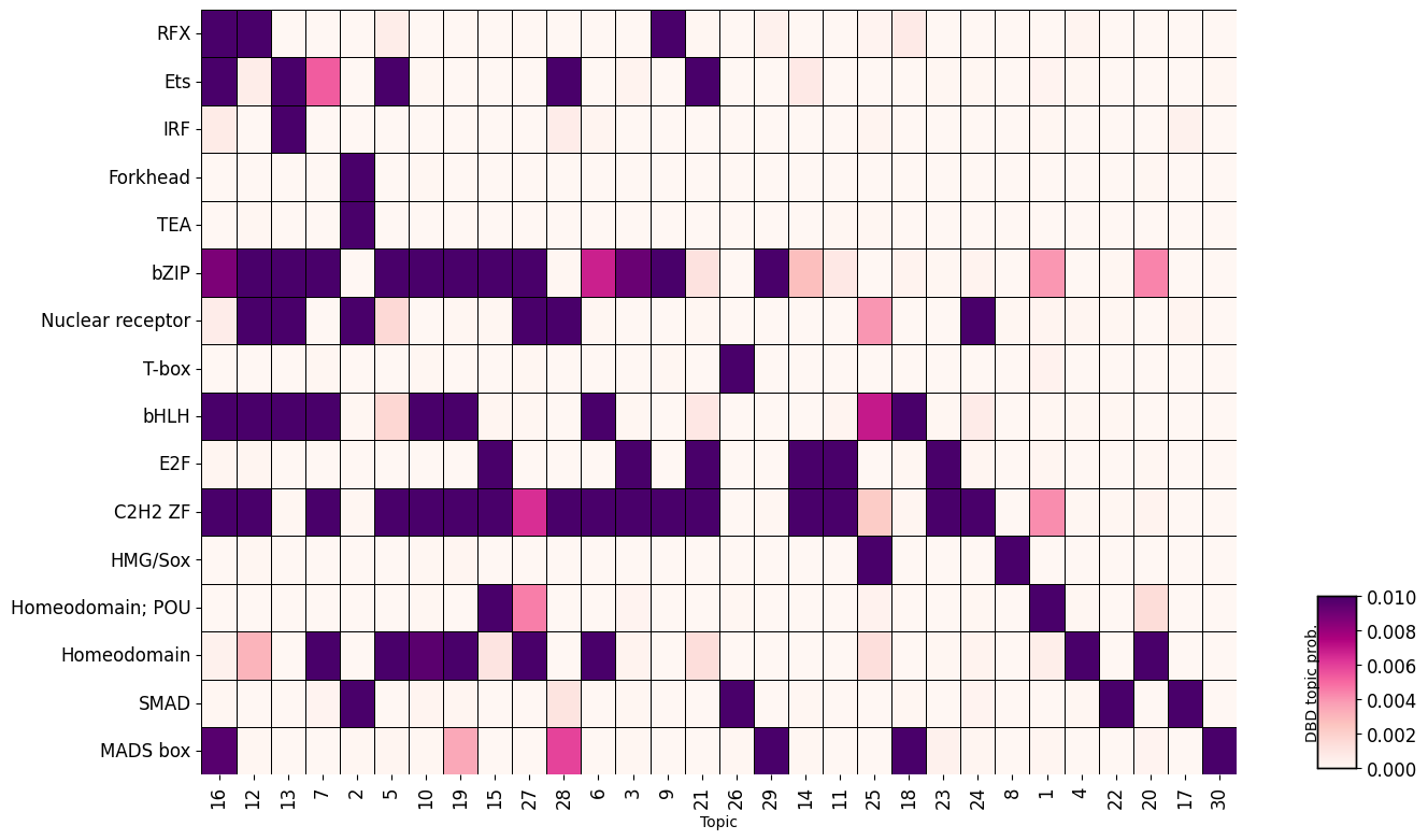
DBD-Topic Heatmap

Visualize the relationship between topics and DNA-binding domains using dbd_topic_heatmap(). This shows us which DBDs often co-occur.

%matplotlib inline
tm.pl.dbd_topic_heatmap(
    adata,
    width=12,
    height=8,
    x_label_rotation=90,
)

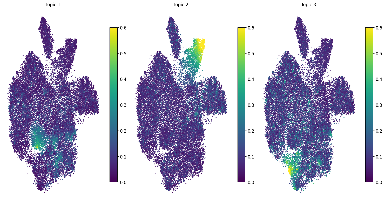
Topic Visualization in t-SNE Space

Plot t-SNE visualization of regions colored by topic probabilities using region_topic_tsne().

# Plot regions colored by dominant topic
tm.pl.region_topic_tsne(adata, topics_to_show=["Topic_1", "Topic_2", "Topic_3"], ncols=3, width=15)

Computing t-SNE coordinates from region-topic matrix...